
Created
Oct 26, 2021 06:41 PM
Topics
+ LSTM
Features of CNN1. Convolution Operation1D ContinuousHyper Parameters2D DiscreteImage Processing KernelsEdge DetectionBlurringHorizontal line detectionVertical line detectionExampleTODO Backpropagation in Convolution Layer2. Pooling/Subsampling LayerMax PoolingExampleAverage PoolingBackpropagation in Pooling Layer3. Convolution Layer and Weight SharingFull Convolutional Neural Network ArchitectureAnalysisOther Types of ClassificationRecurrent Neural NetworksProsIntuitionRecurrent UnitTrainingBack Propagation Through Time: Backward PassLSTM (Long short-term memory)IdeaComposition
Features of CNN
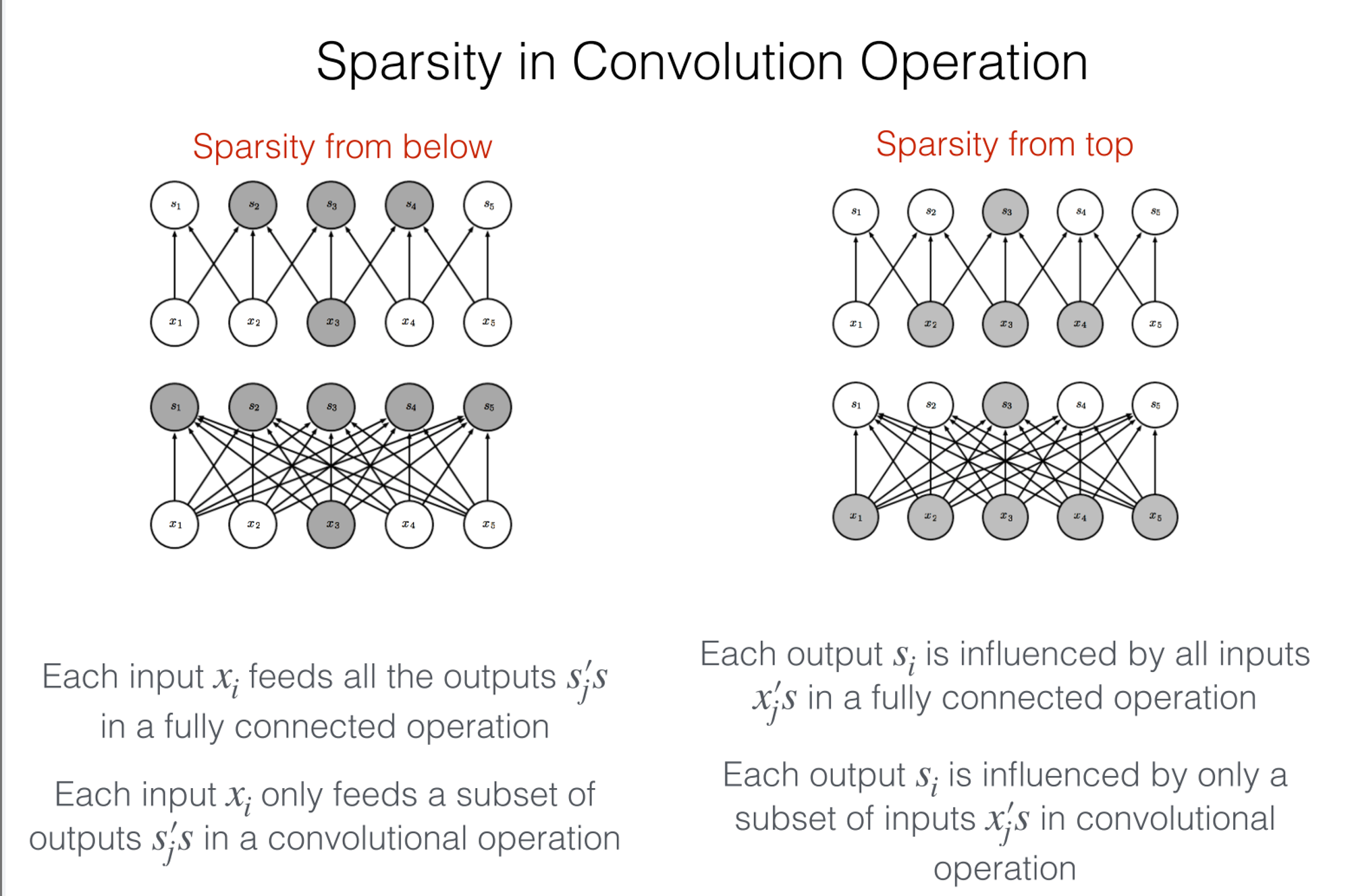
Local receptive fields
Feature pooling
Weight sharing
1. Convolution Operation

1D Continuous
(f * g )(t)=(g * f )(t)
The convolution of the function by the kernel
a part of the convolution function
iteration number
Hyper Parameters

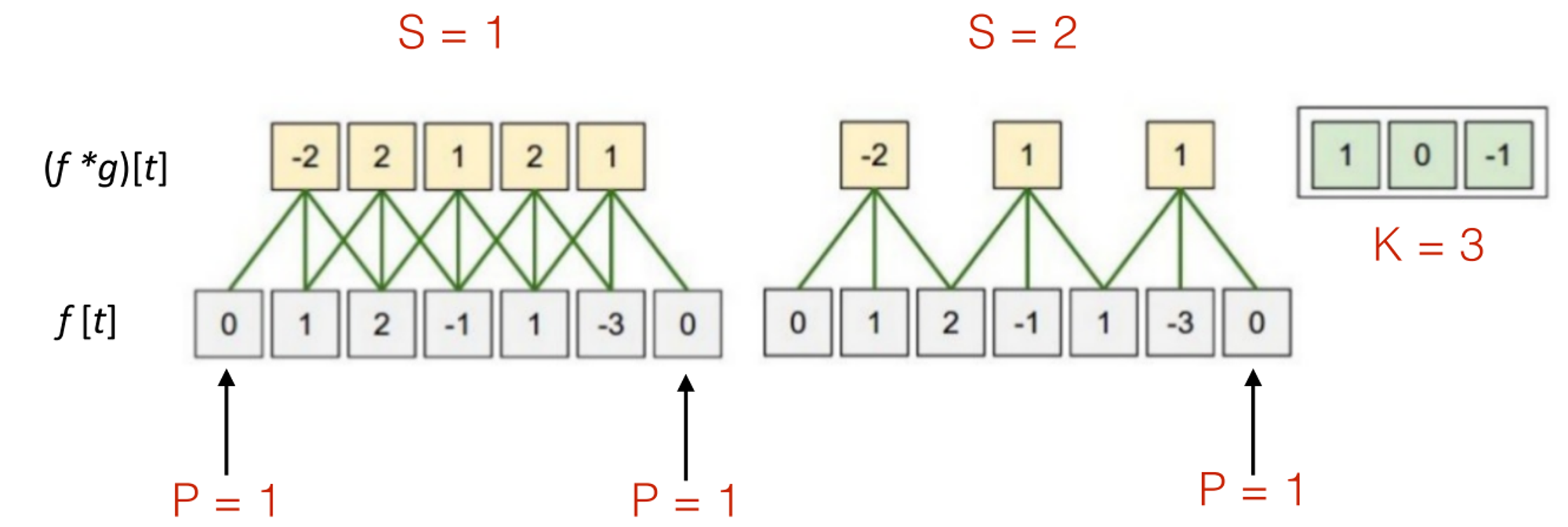
Kernel size : size of the function: how many is used to compute
Stride : skip inputs to compute each convolution
- must <
- Makes more sparse
Input Padding : pad zeros to the beginning & end of
- Reduce edge-effect: left-most & right-most inputs generates a different distribution
- Processing Image: add a border of zeros
2D Discrete


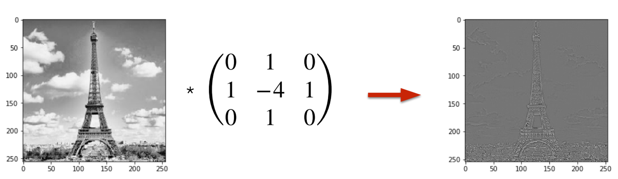
Image Processing Kernels
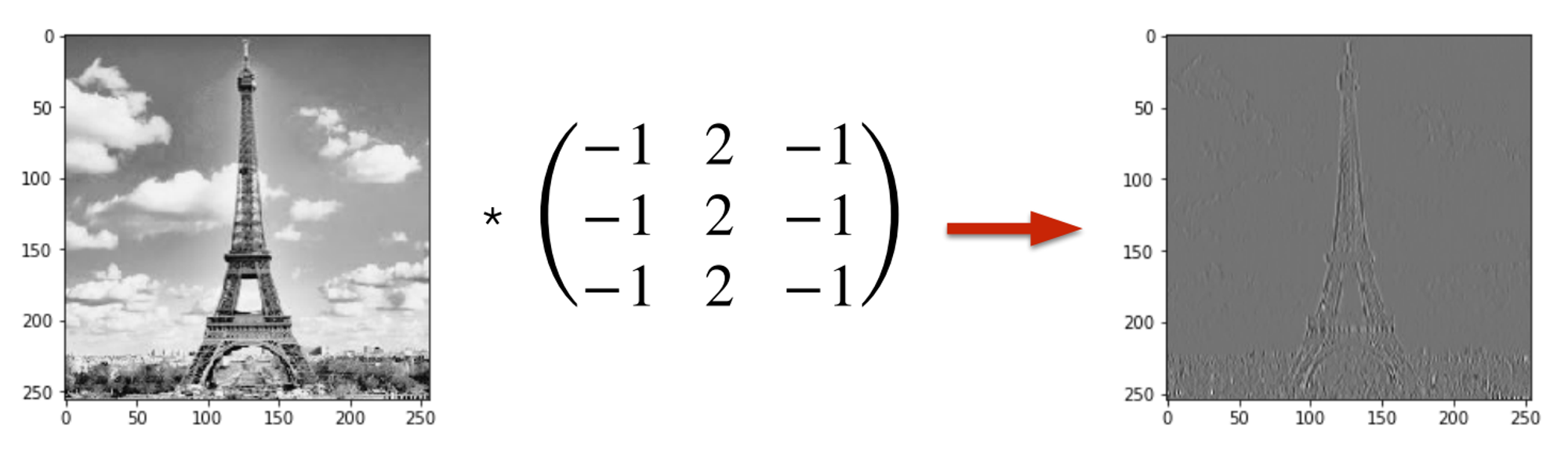
Edge Detection
Edge = gradient of the values of the neighboring pixels
- Similar neighboring pixels → small gradient → not edge
- Different neighboring pixels → large gradient → edge

Blurring

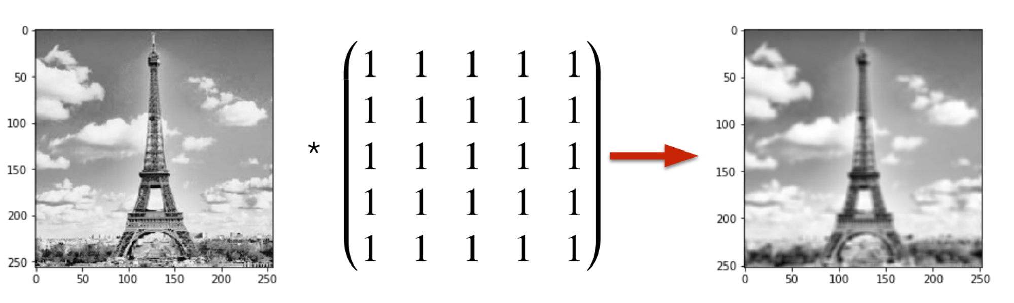
- Large kernel size ⇒ more blurring
Horizontal line detection

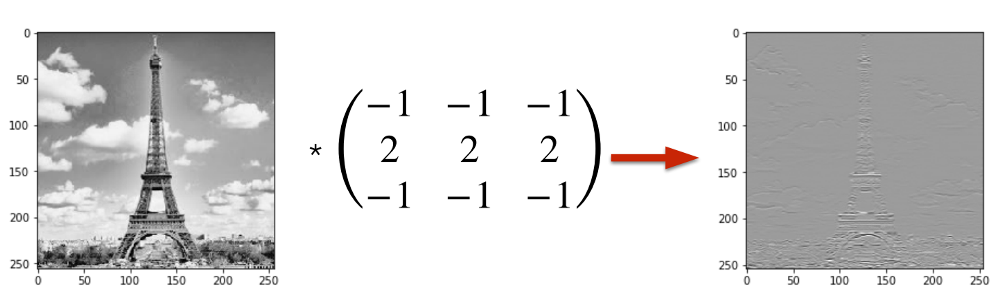
Vertical line detection

Example
Alexnet

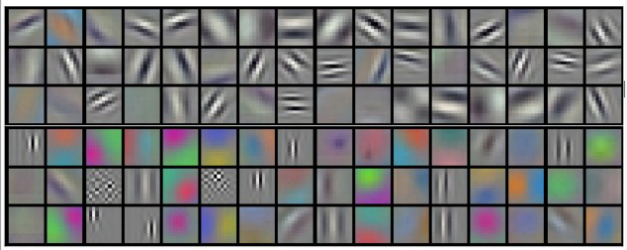
Interpretation: most of them are directing edges at different directions
Randomly initialize kernals
Train the network to optimize the kernels
TODO ‣

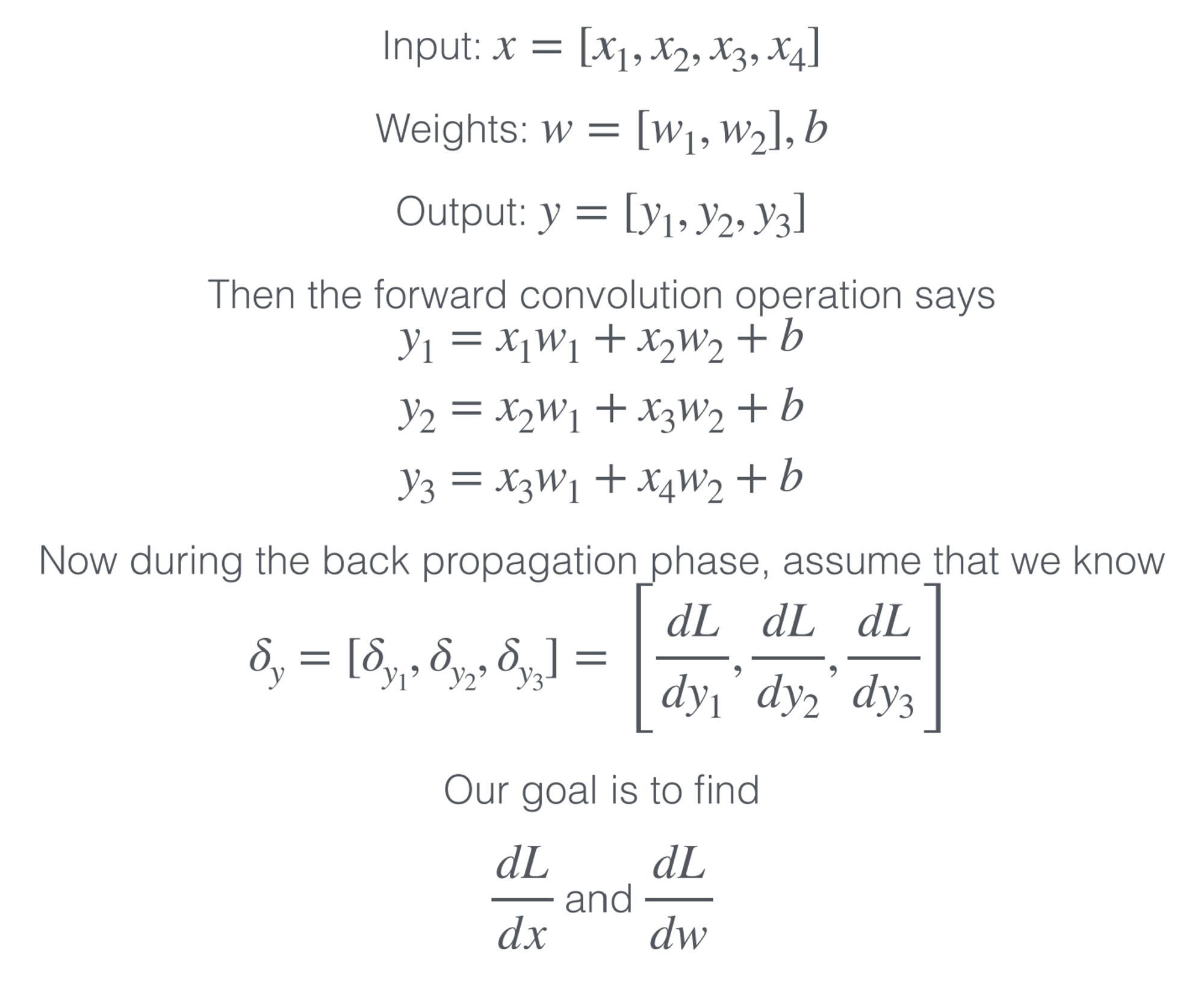
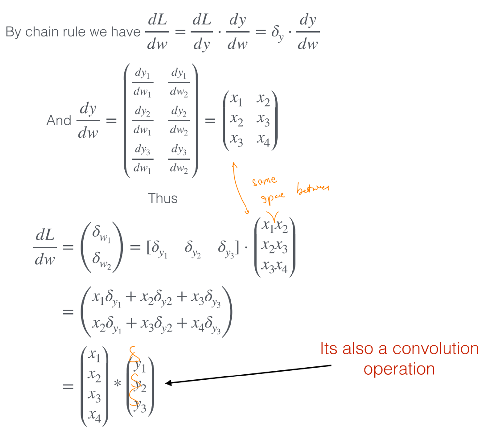
Backpropagation in Convolution Layer
1D Discrete Example
- Weights represents the kernel function


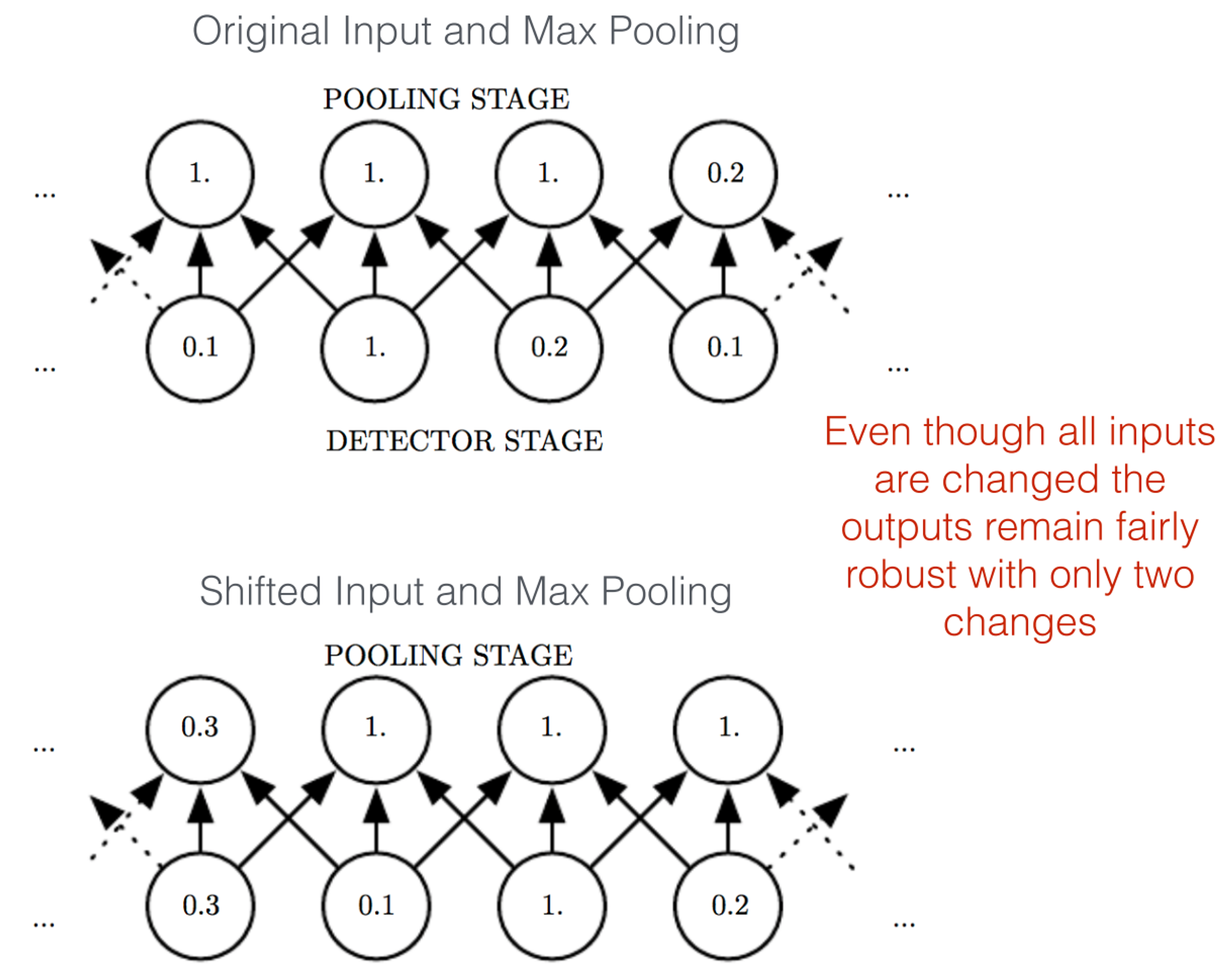
2. Pooling/Subsampling Layer
- Applied after the Convolutional layer
- A simpler convolution operation
- Replace the output at a certain location with the summary statistics of nearby inputs
⇒ Make the network invariant to translation
- Allows us to convert a variable sized input into a fixed size output ⇒ invariance
Max Pooling


Pick the largest in each 2x2 block
- 2x2 filter at stride 2 ⇒ decrease resolution from 4x4 to 2x2
- Hyperparameter: Filter Kernel Size, Stride
Example

Average Pooling
norm of the rectangular neighborhood
- Weighted average based on distance from the center pixel
Backpropagation in Pooling Layer
TBD
3. Convolution Layer and Weight Sharing
Feature maps: generate using kernels
Multiple kernels
Full Convolutional Neural Network Architecture

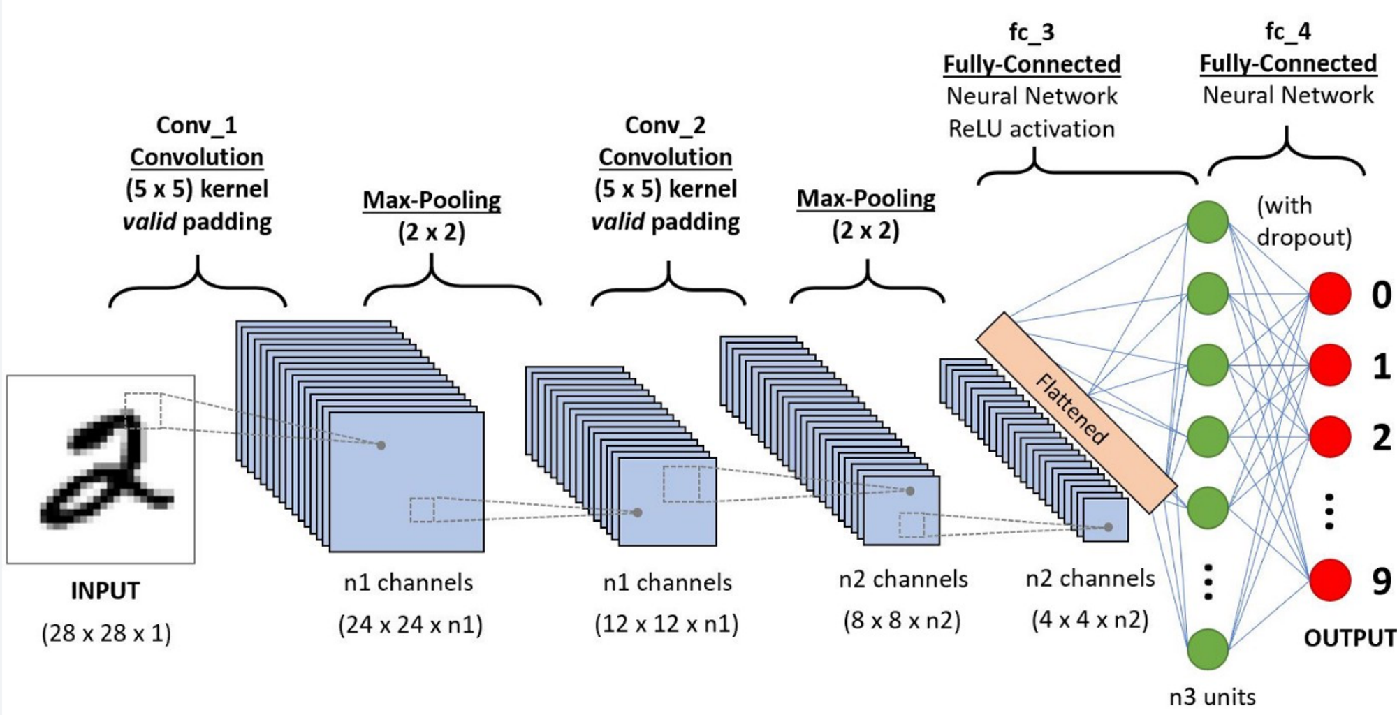
Each feature map can connect to any previous feature maps
- Connection matrix
Analysis
CNN: Good at one-to-one classification
Other Types of Classification
one-to-many: generate captions for a movie, sentiment analysis
many-to-one: sentiment analysis
many-to-many: translation; given a video of variable number of frames, we want to classify each frame?
Recurrent Neural Networks
Pros
- Able to handle variable size inputs & outputs
- Able to handle sequential data
Intuition
Sequentially read from left to right
Maintain an internal memory state
- Captures data seen so far
- Updated with new information
Implementation: Recurrent Relation
Recurrent Unit


Training
Back Propagation Through Time: Backward Pass

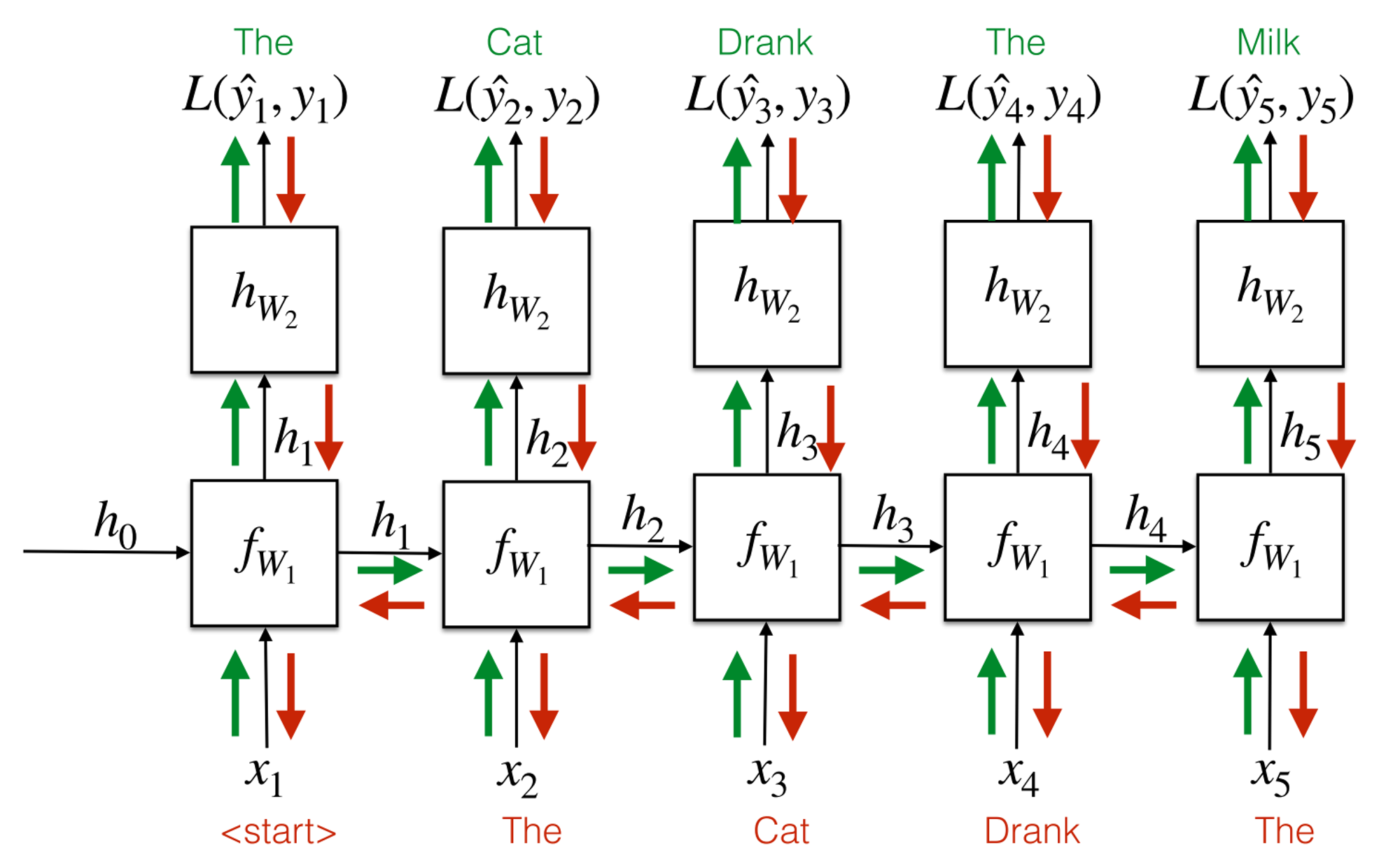
- Take the average of the multiple gradients computed toward in each pass to update
LSTM (Long short-term memory)
Encode "long-term memory" in a cell's state to solve the vanishing gradient problem

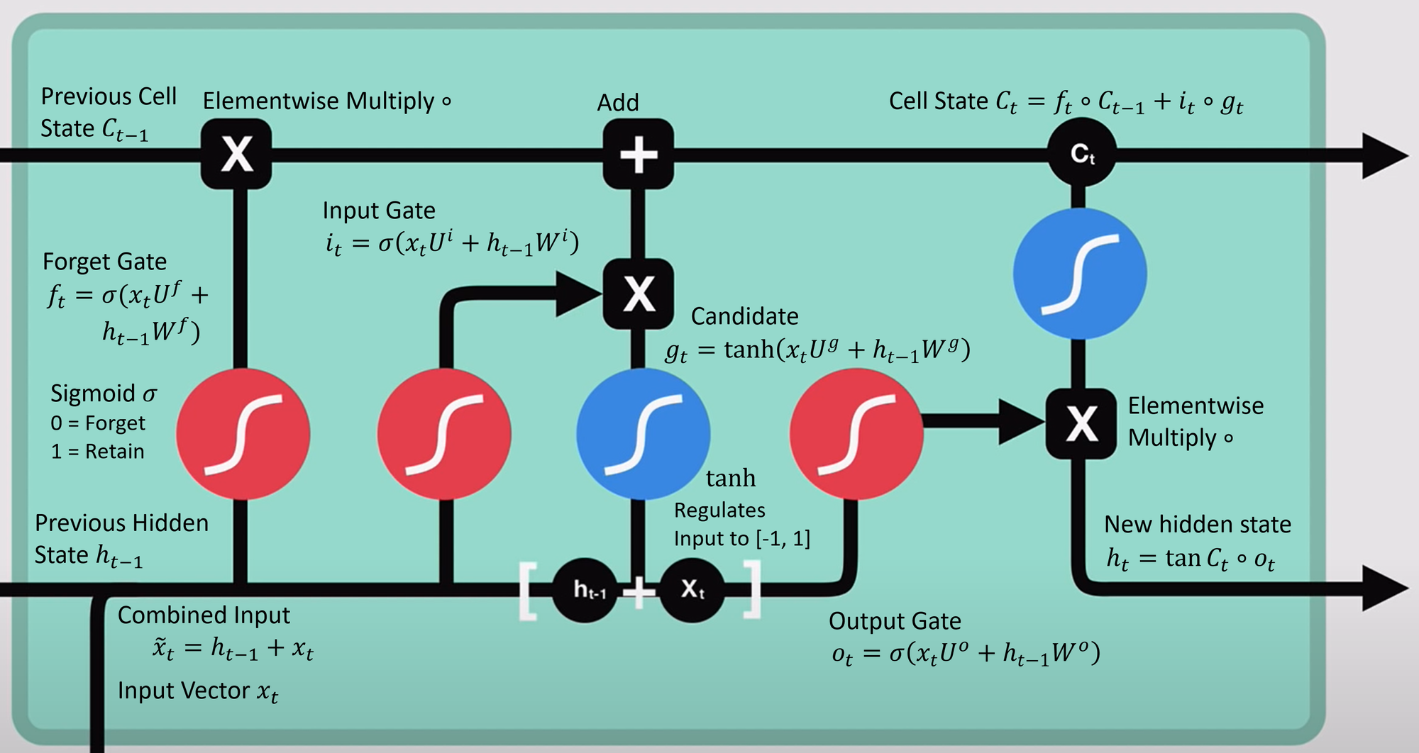
Idea
RNN: keep track of the arbitrary long-term dep input sequence
⇒ back-propagation leads the vanishing/exploding gradient problem
- Vanishingly small ⇒ Stop further training
- Explosively large ⇒
RNN only pass hidden state along the sequence; not good at dealing with long sequences
Composition
embed_size = 32         *# size of the input feature vector representing each word*

hidden_size = 32        *# number of hidden units in the LSTM cell*

num_epochs = 1          *# number of epochs for which you will train your model*

num_samples = 200       *# number of words to be sampled*

batch_size = 20         *# the size of your mini-batch*

seq_length = 30         *# the size of the BPTT window*

learning_rate = 0.002   *# learning rate of the model*

h = batch * hidden
Lab6
Input = batch * ?? * input_size
Output = batch * output_size
Target = batch
ㅤ | Lab6 | HW4 |
Input | batch * ?? * input size | batch * input size |
Embed | ㅤ | input * hidden |
ih | input * hidden | ㅤ |
hh | hidden * hidden | ㅤ |
Output | batch * output size | ㅤ |
Target | batch | batch * input size |